This part of the tutorial shows you how to use EZbakR and the output of fastq2EZbakR to perform an isoform-level analysis of NR-seq data. There are steps to this analysis:
Create EZbakRData object
Estimate TEC fraction news
Estimate isoform fraction news
Linear mixing model using TEC fraction news + isoform abundance estimates
Convert fraction news to rate constants
Average replicate data
Compare kinetic parameter estimates between SMG1i and DMSO samples
This tutorial will also show you how to perform and make use of alternative feature assignment strategies.
Isoform-level analyses
Make sure you have EZbakR installed, then load the following packages to follow all of the steps in this part of the tutorial:
library(data.table)library(dplyr)
Attaching package: 'dplyr'
The following objects are masked from 'package:data.table':

    between, first, last
The following objects are masked from 'package:stats':

    filter, lag
The following objects are masked from 'package:base':

    intersect, setdiff, setequal, union
library(EZbakR)
Quickstart
Here is the code that I will walk through more thoroughly in the following subsections:
The first step of any EZbakR analysis is to create an EZbakRData object, which consists of two components: a cB data frame and a metadf data frame. See the EZbakR docs for more details. There isn’t anything too unique in this case, except I am using some cute tricks to automatically populate the necessary metadf fields, and using data.table to load the cB due to its ultra-fast all purpose file reading function, fread():
You will have to specify the actual path to the cB file (replacing path/to/cB/ with the actual path to that directory created by fastq2EZbakR).
Step 2: Estimate TEC fraction news
The first unique step of an isoform-level analysis is to estimate the fraction of reads in each transcript equivalence class (TEC) that are new. I’ll show the code first and then explain it:
features is set to “XF” (exonic-regions of genes) and “TEC” (transcript equivalence class). The first is technically not necessary, but is included because it is very convenient to associate isoforms with their gene of origin. The second is the key feature in this case.
filter_condition is set to |, which means that if either the XF column or the TEC column is “__no_feature” or NA, that row will get filtered out. The default is that both have to meet this criterion (&).
pold_from_nolabel is a nice way to improve the stability of new and old read mutation rate estimates by using provided -s4U data to estimate the old read mutation rate (pold). It is not strictly necessary but can be useful when mutation rates are low or label times are short.
Step 3: Estimate isoform fraction news
Next is the real special part. EZbakR will combine information about transcript isoform abundances with the TEC fraction new estimates from last step to estimate isoform fraction news. Again, I’ll show the code (with pseudo file paths that you will have to edit) first:
The first part requires you to provide a named vector of paths to all the RSEM isoform quantification files, with each file path named the metadf sample to which it comes from. I am using list.file() for this task, looking for all files in the rsem directory generated by fastq2EZbakR that have “isoform” in their name, which denotes the isoform abundance estimates from RSEM. EZbakR’s ImportIsoformQuant() function then imports this data and adds it to your EZbakRData object.
The second part can typically be run with default options. You may consider changing the TPM_min and count_min (1 and 10 by default) settings, which decides the TPM and expected read count cutoff for isoforms considered “expressed”. Isoforms below these cutoffs get filtered out and will not have their fraction new estimated.
Step 4-6: Estimate, average, and compare rate constants
From here on out, it’s a standard EZbakR analysis:
ezbdo <-EstimateKinetics(ezbdo, features ="transcript_id",exactMatch =FALSE)ezbdo <-AverageAndRegularize(ezbdo, features ="transcript_id",exactMatch =FALSE)ezbdo <-CompareParameters(ezbdo,features ="transcript_id",design_factor ="treatment",reference ="DMSO",experimental ="SMG1i",exactMatch =FALSE)
You now have two different fractions tables in your EZbakRData object, so in the first step (EstimateKinetics()) you need to specify that you want the table with the feature column “transcript_id”. Setting exactMatch to FALSE prevents you from having to specify all of the features in this table (XF being the other one). I have included features = "transcript_id" for completeness, but it is technically overkill at this point as there is only one table of each relevant kind at each step if you have done everything as shown in this tutorial so far.
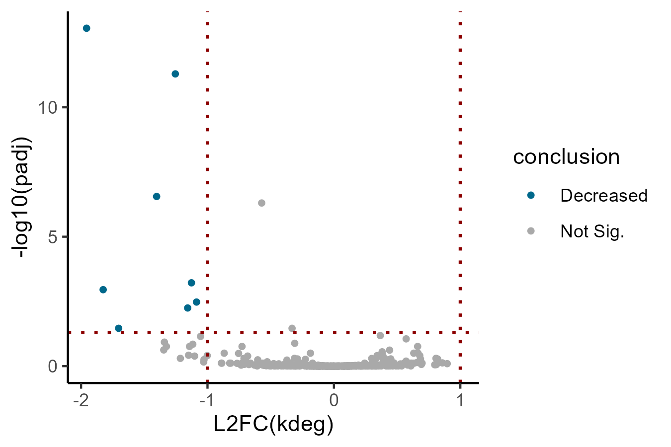
You can explore the output and see the stabilization of the PTC-containing SRSF3 isoform (but not the major isoform) like so:
Isoform-level analyses are powerful strategies by which to assess the kinetics for the actual RNA species that are synthesized and degraded. That being said, for these analyses to be accurate, your annotation of expressed isoforms must be accurate. This is often difficult in practice, with troublesome, poorly annotated loci an inevitability. It can thus be nice to have ways to orthogonally validate what you are seeing by the transcript isoform level analysis.
Enter alternative feature sets. In the fastq2EZbakR analysis, I included exon bin and exon-exon junction feature assignments, as these are both powerful options for this task. Exon-exon junction analyses can identify specific spliciing events that are correlated with a change in RNA stability, regardless of whether the full isoform splice graphs are accurate, and exon bin analyses can identify exonic regions that show strong stabilization signal. Both can be used in this case to corroborate the SRSF3 stabilization event.
How?
Reads will often map to several exon bins and/or exon-exon junctions. Thus, dealing with these requires some slight alterations to EstimateFractions.
Of note are the split_multi_features and multi_feature_cols options. This will copy the data for reads mapping to multiple instances of a given feature (e.g., multiple exon bins) so that fraction news are estimated for each instance of a given feature. The junction-level analysis is similar, except that there are two junction-related features: