EZbakR for people in a hurry • EZbakR

Abstract

EZbakR is a one-stop-shop for analyses of nucleotide recoding RNA-seq datasets (NR-seq). NR-seq refers to a class of methods (e.g., TimeLapse-seq, SLAM-seq, TUC-seq, etc.) that combine RNA-seq, metabolic labeling, and unique metabolic label recoding chemistries. These methods were originally developed to dissect the kinetics of RNA synthesis and degradation. Excitingly though, a treasure trove of extensions of the original methods have been created over the years. To-date, nucleotide recoding has been combined with TT-seq, Start-seq, Ribo-seq, scRNA-seq, Perturb-seq, and subcellular fractionation, just to name a few such extensions. In addition, while the original methods used 4-thiouridine (s⁴U), the same chemistry has been found to work with 6-thioguanosine (s⁶G), opening the door to dual-labeling experimental designs (e.g., TILAC). EZbakR was designed to facilitate anlayses of the full gamut of NR-seq methods. While not all analyses implemented in EZbakR can be applied to all variants of NR-seq, EZbakR’s modular design means that it has something for everyone. In this vignette, we will quickly highlight the main modules of EZbakR. For simplicity, we will be focusing on how to perform a standard, single-label NR-seq analysis. Other vignettes go into greater detail about each module and the broad array of analyses that can be performed by each.

Necessary Setup

You will need to install and load EZbakR. Instructions to do so can be found at this link. Setting the seed will also ensure exact reproducibility of analyses of simulated data shown in this vignette. Finally, I will use a little bit of dplyr to showcase some key results:

library(EZbakR)
library(dplyr)
#> 
#> Attaching package: 'dplyr'
#> The following objects are masked from 'package:stats':
#> 
#>     filter, lag
#> The following objects are masked from 'package:base':
#> 
#>     intersect, setdiff, setequal, union
set.seed(42)

Step 0: Create an EZbakRData Object

To use EZbakR, you will need to create an EZbakRData object. An EZbakRData object consists of two components: a cB data frame and a metadf data frame. cB stands for “counts binomial” and contains all of the information about mutations seen in sequencing reads in each sample sequenced. metadf stands for “metadata data frame” and contains information about the experimental details of each sample (i.e., how long the metabolic label feed was). Examples of what these data structures look like are lazily loaded when you load EZbakR. This means that you can call them as if you created them yourselves, with example_cB and example_metadf:

# Check out examples:
example_cB
example_metadf

A cB data frame consists of rows corresponding to groups of reads with identical data, where data corresponds to the:

Sample of origin. This should be noted in the sample column of the cB.
Mutational content. This should be noted by one or more columns of the form (e.g., TC in example_cB). The value in these columns should correspond to the observed number of mutations.
Mutable nucleotide content. This should be noted by one or more columns of the form n (e.g., nT in example_cB). The value in these columns should correspond to the number of mutable bases overlapped by the read.
Genomic features the read was assigned to. In EZbakR, these can be named anything. The fastq2EZbakR pipeline most commonly paired with EZbakR can include feature columns such as those which show up in example_cB:
- GF: Stands for “gene feature” and represents the gene (exonic or intronic regions) the read overlapped
- XF: Stands for “exonic feature” and represents the gene (exonic regions only) the read overlapped
- rname: Chromosome the read came from.

The final column of the cB data frame is n, the number of reads with identical data for the other columns. cB data frames are most easily obtained from the Snakemake pipeline fastq2EZbakR, available here.

A metadf table has the following required columns:

sample: Sample name, as it shows up in the cB table.
Metabolic label time information. If you have a single label, this should be documented in a column called tl. If you used multiple labels, then the different label times should be noted in a column called tl_, where denotes the type of mutation that conversion of the label yields. For example, if you are using s⁴U (conversion yields T-to-C mutations) and s⁶G (conversion yields G-to-A mutations), then your metadf should include columns tl_TC and tl_GA.

The remaining columns can be named anything you want and should describe aspects of each experiment. NOTE: these are currently exclusively interpreted as discrete factors. Things like time-series modeling is not currently supported, but may be in future releases. These factors will be used when deciding how to group samples when averaging replicate data and performing comparative analyses. More on this later!

Once you have a cB and metadf table, you can create an EZbakRData object:

ezbdo <- EZbakRData(example_cB, example_metadf)

Now, let’s generate some simulated data to be used in the remaining steps:

# Simulate 500 "genes" worth of data
  # Simulates 2 replicates of 2 different experimental conditions
simdata <- EZSimulate(nfeatures = 500, nreps = 2)

ezbdo <- EZbakRData(simdata$cB, simdata$metadf)

Step 1: EstimateFractions()

The first step of any NR-seq analysis is to figure out what fraction of your reads come from each expected mutational population. For example, in a standard s⁴U labeling NR-seq experiment, you will have reads from a high T-to-C mutation population and reads from a low T-to-C mutation population. Technically, this involves two steps: 1) estimating mutation rates of the two populations in each labeled sample and 2) estimating fractions. Both of these steps are performed with a single function in EZbakR: EZbakRFractions():

ezbdo <- EstimateFractions(ezbdo)
#> Estimating mutation rates
#> Summarizing data for feature(s) of interest
#> Averaging out the nucleotide counts for improved efficiency
#> Estimating fractions
#> Processing output

See ?EstimateFractions() for details and descriptions of optional parameters. We can use the simulated ground truth to assess estimate accuracy and confirm that the method is working:

# Simulated ground truth
truth <- simdata$PerRepTruth

# Get fraction estimates. 
  # Can also access with ezbdo$fractions[[1]] or ezbdo$fractions$feature
est <- EZget(ezbdo, type = 'fractions')

# Combine
compare <- dplyr::inner_join(est, truth, by = c('sample', 'feature'))

# Assess accuracy
plot(compare$true_fraction_highTC, compare$fraction_highTC)
abline(0,1)

Looks good!

Step 2: EstimateKinetics()

The next step of a standard NR-seq analysis is to use the estimates of mutational population proportions (and possibly normalized read counts) to estimate kinetic parameters of interest (e.g., degradation and synthesis rate constants). The simplest and quickest way to do this is with EstimateKinetics():

ezbdo <- EstimateKinetics(ezbdo)

By default, this uses a standard, steady-state, single rate constant model of RNA metabolism to infer a degradation rate constant (kdeg) and synthesis rate constant (ksyn) for each gene. Other analysis strategies implemented in EstimateKinetics() include those more appropriate for non-steady-state systems or short label times. The strategy argument in EstimateKinetics() sets which analysis strategy is used. See ?EstimateKinetics for details.

Again, let’s compare to ground_truth:

# Simulated ground truth
truth <- simdata$PerRepTruth

# Get fraction estimates. 
  # Can also access with ezbdo$fractions[[1]] or ezbdo$fractions$feature
est <- EZget(ezbdo, type = 'kinetics')

# Combine
compare <- dplyr::inner_join(est, truth, by = c('sample', 'feature'))

# Assess accuracy
plot(log(compare$true_kdeg), compare$log_kdeg)
abline(0,1)

Great!

Step 3: AverageAndRegularize()

Typically, you will have multiple replicates of each experimental condition. In that case, the next step is to average the data across these replicates and estimate overall uncertainties. This can then be passed along to downstream comparative analyses to see which features have differences in their kinetic parameters between different experimental conditions. This averaging process is done with AverageAndRegularize():

ezbdo <- AverageAndRegularize(ezbdo,
                              parameter = "log_kdeg")
#> Fitting linear model
#> Estimating coverage vs. variance trend
#> Regularizing variance estimates

See ?AverageAndRegularize() for details. One cool thing about AverageAndRegularize() is that it implements a heteroskedastic linear model and can thus be passed formula objects to detail how you would like to stratify samples, and whether or not there are any batches you would like to regress out of the main parameter effects. See the relevant vignette for more details.

Finally, setting parameter = "log_kdeg" was not technically necessary as it is the default, but it showcases that you need to specify which kinetic parameter you want to average across replicates. If you run this again with a different parameter, a new table will be added to the ezbdo$averages list:

ezbdo <- AverageAndRegularize(ezbdo,
                              parameter = "log_ksyn")
#> Fitting linear model
#> Estimating coverage vs. variance trend
#> Regularizing variance estimates

Let’s make sure the estimates are still accurate:

truth <- simdata$AvgTruth

est <- EZget(ezbdo, type = 'averages', parameter = 'log_kdeg')

compare <- dplyr::inner_join(truth, est, by = 'feature')

plot(compare$true_logkdeg_treatmenttreatment1,
     compare$mean_treatmenttreatment1)
abline(0,1)

All good!

Step 4: CompareParameters()

Once you have replicate averaged parameter estimates, you can compare them and assess the “statistical significance” of any observed differences. This is done with CompareParameters():

ezbdo <- CompareParameters(ezbdo,
                           condition = 'treatment',
                           reference = 'treatment1',
                           experimental = 'treatment2',
                           parameter = "log_kdeg")

In addition to providing the EZbakRData object output by AverageAndRegularize(), you also need to specify three other arguments:

condition: the metadf column (or function of columns) that replicates were stratified by. The simulated metadf has a single experimental detail column called treatment, so this is the condition here.
reference: what value of condition do you want to consider the “reference” level.
experimental: what value of condition do you want to consider the “experimental” level.

Once again, parameter’s default value is “log_kdeg”, but is specified here to be explicit.CompareParameters() will calculate the difference in average parameter as: experimental - reference.

EZbakR provides some convenient visualization functions to inspect the output of CompareParameters().

Volcano plot:

EZVolcanoPlot(ezbdo, parameter = "log_kdeg",
              condition = 'treatment',
              reference = 'treatment1',
              experimental = 'treatment2')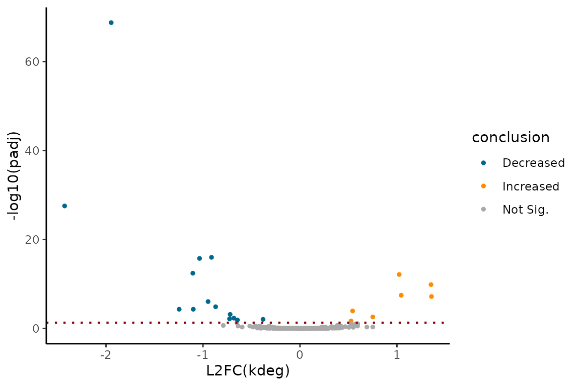

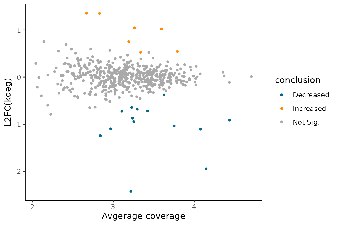
MA plot:

EZMAPlot(ezbdo, parameter = "log_kdeg",
         condition = 'treatment',
         reference = 'treatment1',
         experimental = 'treatment2')