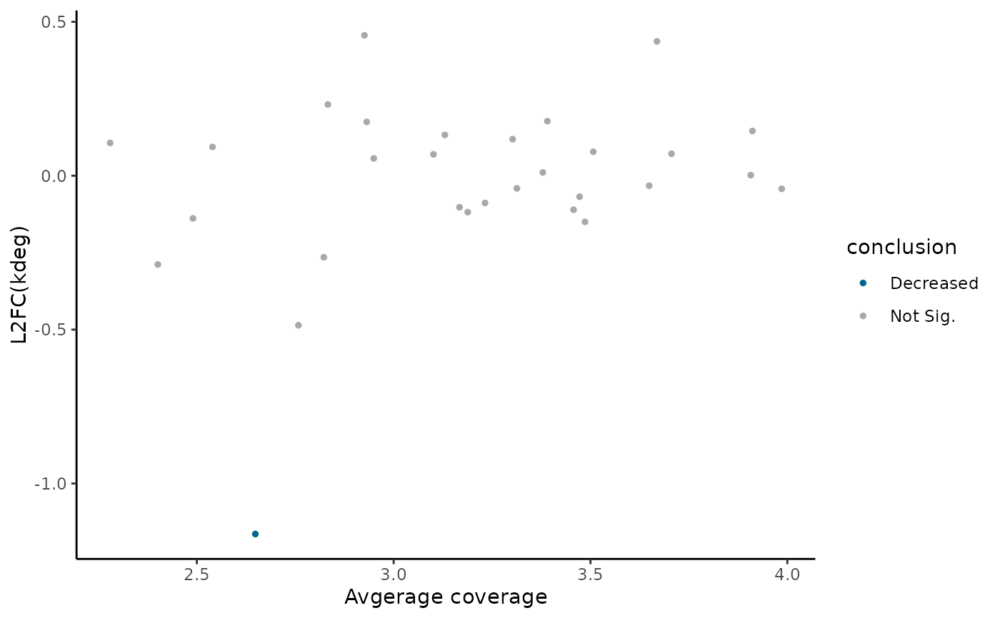
Make an MAPlot from EZbakR comparison

Make a plot of effect size (y-axis) vs. log10(read coverage) (x-axis), coloring points by position relative to user-defined decision cutoffs.

Usage

EZMAPlot(
  obj,
  parameter = "log_kdeg",
  design_factor = NULL,
  reference = NULL,
  experimental = NULL,
  param_name = NULL,
  param_function = NULL,
  features = NULL,
  condition = NULL,
  repeatID = NULL,
  exactMatch = TRUE,
  plotlog2 = TRUE,
  FDR_cutoff = 0.05,
  difference_cutoff = log(2),
  size = NULL
)

Arguments

obj: An object of class EZbakRCompare, which is an EZbakRData object on which you have run CompareParameters
parameter: Name of parameter whose comparison you want to plot.
design_factor: Name of factor from metadf whose parameter estimates at different factor values you would like to compare.
reference: Name of reference condition factor level value.
experimental: Name of condition factor level value to compare to reference.
param_name: If you want to assess the significance of a single parameter, rather than the comparison of two parameters, specify that one parameter's name here.
param_function: NOT YET IMPLEMENTED. Will allow you to specify more complicated functions of parameters when hypotheses you need to test are combinations of parameters rather than individual parameters or simple differences in two parameters.
features: Character vector of feature names for which comparisons were made.
condition: Defunct parameter that has been replaced with design_factor. If provided gets passed to design_factor if design_factor is not already specified.
repeatID: If multiple kinetics or fractions tables exist with the same metadata, then this is the numerical index by which they are distinguished.
exactMatch: If TRUE, then features and populations have to exactly match those for a given fractions table for that table to be used. Means that you can't specify a subset of features or populations by default, since this is TRUE by default.
plotlog2: If TRUE, assume that log(parameter) difference is passed in and that you want to plot log2(parameter) difference.
FDR_cutoff: False discovery cutoff by which to color points.
difference_cutoff: Minimum absolute difference cutoff by which to color points.
size: Size of points, passed to geom_point() size parameter. If not specified, a point size is automatically chosen.

Value

A ggplot2 object. Y-axis = log2(estimate of interest (e.g., fold-change in degradation rate constant); X-axis = log10(average normalized read coverage); points colored by location relative to FDR and effect size cutoffs.

Details

EZMAPlot() accepts as input the output of CompareParameters(), i.e., an EZbakRData object with at least one "comparisons" table. It will plot the "avg_coverage" column in this table vs. the "difference" column. In the simplest case, "difference" represents a log-fold change in a kinetic parameter (e.g., kdeg) estimate. More complicated linear model fits and comparisons can yield different parameter estimates.

NOTE: some outputs of CompareParameters() are not meant for visualization via an MA plot. For example, when fitting certain interaction models, some of the parameter estimates may represent average log(kinetic paramter) in one condition. See discussion of one example of this here.

EZbakR estimates kinetic parameters in EstimateKinetics() and EZDynamics() on a log-scale. By default, since log2-fold changes are a bit easier to interpret and more common for these kind of visualizations, EZMAPlot() multiplies the y-axis value by log2(exp(1)), which is the factor required to convert from a log to a log2 scale. You can turn this off by setting plotlog2 to FALSE.

Examples


# Simulate data to analyze
simdata <- EZSimulate(30)

# Create EZbakR input
ezbdo <- EZbakRData(simdata$cB, simdata$metadf)

# Estimate Fractions
ezbdo <- EstimateFractions(ezbdo)
#> Estimating mutation rates
#> Summarizing data for feature(s) of interest
#> Averaging out the nucleotide counts for improved efficiency
#> Estimating fractions
#> Processing output

# Estimate Kinetics
ezbdo <- EstimateKinetics(ezbdo)

# Average estimates across replicate
ezbdo <- AverageAndRegularize(ezbdo)
#> Fitting linear model
#> Estimating coverage vs. variance trend
#> Regularizing variance estimates

# Compare parameters across conditions
ezbdo <- CompareParameters(
ezbdo,
design_factor = "treatment",
reference = "treatment1",
experimental = "treatment2"
)

# Make MA plot (ggplot object that you can save and add/modify layers)
EZMAPlot(ezbdo)